In what units is the modulus of elasticity measured?

An indicator of the incompressibility/resistance to compressibility of a substance.

Illustration of uniform compression

Bulk modulus of elasticity

(or) of a substance is a measure of how resistant to compression that substance is.
It is defined as the ratio of the infinitesimal increase in pressure to the resulting relative
decrease in volume. [1] Other moduli describe the response of a material (strain) to other types of stress: the shear modulus describes the response to shear, and Young's modulus describes the response to linear stress. For a liquid, only the bulk modulus of elasticity matters. For a complex anisotropic solid such as K {\displaystyle K}B{\displaystyle B}wood or paper, these three modules do not contain enough information to describe its behavior, and Hooke's full generalized law must be used.

Definition[edit]

The bulk modulus of elasticity can be formally defined by the equation K > 0 {\displaystyle K>0}

K = − V d p d V {\displaystyle K=-V{\frac {dP}{dV))}

where is pressure, is the initial volume of the substance, and denotes the derivative of pressure with respect to volume. Given a unit of mass, P {\displaystyle P}V{\displaystyle V}d P/d V{\displaystyle dP/dV}

K = ρ d p d ρ {\displaystyle K=\rho {\frac {dP}{d\rho))}

where ρ

is the initial density, and d
P
/ d
ρ
denotes the derivative of pressure with respect to density (i.e., the rate of change of pressure depending on volume). The inverse bulk modulus gives the compressibility of a substance.

Thermodynamic relation[edit]

Strictly speaking, the bulk modulus of elasticity is a thermodynamic quantity, and in order to specify the bulk modulus, it is necessary to indicate how the pressure changes during compression: constant temperature (isothermal), constant entropy (isentropic), and other variations are possible. . Such differences are especially relevant for gases. K T {\displaystyle K_{T))KS {\displaystyle K_{S))

For an ideal gas, the isentropic process has:

p V γ = c o p s t . ⇒ p ∝ ( 1 V ) γ ∝ ρ γ , {\displaystyle PV^{\gamma }=const. \,\Rightarrow P\propto\left({\frac {1}{V}}\right)^{\gamma}\propto\rho^{\gamma},}

therefore the isentropic bulk modulus is defined as: KS {\displaystyle K_{S))

KS = γ n . {\displaystyle K_{S}=\gamma P.}

Similarly, an isothermal ideal gas process has:

p V = c o p s t . ⇒ p ∝ 1 V ∝ ρ , {\displaystyle PV=const.\,\Rightarrow P\propto {\frac {1}{V}}\propto \rho ,}

therefore, the isothermal modulus of bulk elasticity is given by KT {\displaystyle K_{T}}

KT = P {\displaystyle K_{T}=P}

where γ

is the ratio of heat capacity and
p
is pressure.

When the gas is not ideal, these equations give only an approximation of the bulk modulus. In a liquid, the bulk modulus K

and density
ρ
determine the speed of sound
c
(pressure waves) according to the Newton-Laplace formula
c = K ρ.
{\displaystyle c={\sqrt {\frac {K}{\rho }}}.} In solids and have very similar values. Solids can also withstand shear waves: these materials require one additional elastic modulus, such as a shear modulus, to determine the wave speed. KS {\displaystyle K_{S}} KT {\displaystyle K_{T}}

General concepts

The modulus of elasticity (Young's modulus) is an indicator of the mechanical property of a material, characterizing its resistance to tensile deformation . In other words, this is the value of the ductility of the material. The higher the elastic modulus values, the less any rod will stretch under other equal loads (sectional area, load magnitude, etc.).

Young's modulus in the theory of elasticity is denoted by the letter E. It is a component of Hooke's law (on the deformation of elastic bodies). This value relates the stress arising in the sample and its deformation.

This value is measured according to the standard international system of units in MPa (Megapascals) . But in practice, engineers are more inclined to use the kgf/cm2 dimension.

This indicator is determined empirically in scientific laboratories. The essence of this method is the tearing of dumbbell-shaped samples of material using special equipment. Having found out the elongation and tension at which the sample failed, divide the variable data into each other. The resulting value is the (Young's) modulus of elasticity.

In this way, only the Young’s modulus of elastic materials is determined: copper, steel, etc. And brittle materials are compressed until cracks appear: concrete, cast iron and the like.

Selected values ​​[edit]

Approximate bulk modulus (K) for common materials

The effect of additives of selected glass components on the bulk modulus of a certain base glass. [4]

A material with a bulk modulus of 35 GPa loses one percent of its volume when exposed to an external pressure of 0.35 GPa (~3500 bar).
Approximate bulk modulus (K) for other substances

Physical properties of liquids

Chapter 1. BASICS OF HYDROSTATICS

The main physical properties of a liquid are: fluidity, density, specific gravity, viscosity, compressibility, thermal expansion.

The density of a liquid is a physical quantity numerically equal to the ratio of the mass of a liquid to its volume.

(1.1)

where r

– liquid density,
kg
/
m3
;

m

– mass of liquid;
kg
;

W

– volume of liquid,
m3
.

Specific gravity is a physical quantity numerically equal to the ratio of the weight of a liquid to its volume.

(1.2)

where g

– specific gravity of the liquid,
N
/
m3
;

G

– liquid weight

, N.

Between specific gravity g

and density
r
there is a dependence

(1.3

where g

= 9.81
m
/
s
2 – free fall acceleration.

r values

and
g
for water and some other liquids at different temperatures are given in Appendix 1.

Viscosity is the property of a liquid to resist relative shear of adjacent layers. Viscosity is characterized by dynamic viscosity coefficients m

,
Pa×s
, and
kinematic viscosity n
,
m
/
s
. There is a relationship between these coefficients

(1.4)

The values ​​of the coefficients of dynamic and kinematic viscosity for some liquids are given in Appendix 2.

Compressibility is the property of a liquid to change its volume when pressure changes. Compressibility is characterized by the volumetric compression ratio b

w, which can be determined by the formula

(1.5)

where b

w – volumetric compression ratio, 1/
Pa
;

W

– initial volume of liquid,
m3
;

D W

– change in liquid volume,
m
3;

D p

– change in pressure,
Pa
.

The reciprocal of the volumetric compression ratio is called the volumetric modulus of elasticity K

.
The bulk modulus is measured in Pa
.

(1.6)

The volumetric compression coefficients of liquids change little with changes in temperature and pressure. The values ​​of volumetric compression coefficients and elastic moduli for some liquids are given in Appendix 3.

Thermal expansion is the property of a liquid to change its volume when the temperature changes. Thermal expansion is characterized by the coefficient of thermal expansion , which can be determined from the expression

(1.7)

where is the coefficient of thermal expansion, 1/ K

;

W

– initial volume of liquid,
m3
;

– change in liquid volume, m

3;

– temperature change, K

.

Thermal expansion coefficients for some liquids are given in Appendix 4.

Tasks

1.1. Determine the mass of water in a sleeve with a diameter of 51 mm

and 20
m long.
Solution. The mass of water is determined from formula (1.1)

Density of water according to Appendix 1

Water volume

Then

1.2. Determine the weight of water in hoses with a diameter of 66 mm

and 77
mm
and length 20
m
.

1.3. Determine the mass of diesel fuel oil contained in a tank with a volume of 50 m3

3, if the density of the fuel oil is 920
kg
/
m3
.

1.4. Determine how much volume oil with a mass of 20×103 kg

and density 900
kg
/
m3
.

1.5. Determine the density of petroleum products if their mass is 17.5×103 kg

, volume 20
m3
.

1.6. Determine the weight of ethyl alcohol in a volume of 20 liters.

1.7. Fuel oil level in a vertical cylindrical tank with a diameter of 2 m

dropped by 0.5
m
.
Determine the mass of consumed fuel oil if its density at a temperature of 20 ° C
is 990
kg
/
m3
.

1.8. During hydraulic tests, water leakage is allowed, which should not exceed 3 liters

per square meter of wetted surface.
Is it possible to put into operation a rectangular reservoir with dimensions in plan of 12´6 m

m
to 3.48
m
in one day ? Determine the mass of lost water.

Solution . The volume of lost water was

Mass of lost water

Wetted surface area

Water leakage from one square meter of wetted surface during hydraulic tests

which exceeds the established norm.

1.9. Determine whether it is possible to put into operation a cylindrical tank with a diameter of 12 m

, in which the water level dropped from 5
m
to 4.985
m
.

1.10. Determine the maximum mass of water lost in one day as a result of hydraulic tests of a cylindrical tank with a diameter of 18 m

.
Determine the maximum reduction in water level if the initial level was 3.9 m
.

1.11. Determine the coefficient of dynamic viscosity of oil if the coefficient of kinematic viscosity is 0.624×10-4 m

2/
s
.
Oil density 750 kg
/
m3
.

1.12. Fire water conduit with a diameter of 300 mm

and 50
m
, prepared for hydraulic tests, filled with water at atmospheric pressure.
Determine the volume of water that needs to be additionally supplied to the water pipeline so that the excess pressure in it rises to 5 MPa
. Neglect the deformation of the water supply pipes.

Solution . From equation (1.5) we find that the volume of water that needs to be additionally supplied to the water pipeline is determined as

Volumetric compression ratio of water

Initial volume of water

Then

1.13. During hydraulic testing of a process pipeline 200 m

and with a diameter of 250
mm
, filled with kerosene, the pressure was raised to 1.5
MPa
.
After one hour, the pressure dropped to 1.0 MPa
.
Determine the volume of kerosene leaked through the leak. Take the volumetric compression ratio of kerosene = 80×10-11 1/ Pa
. Neglect pipeline deformation.

1.14. The pressure gauge on a process tank completely filled with oil shows 0.5 MPa

.
When 40 liters
of oil were released, the pressure gauge readings dropped to 0.1
MPa
. Determine the volume of the container if the volumetric compression ratio of oil = 80 × 10-11 1/Pa.

1.15. In a vertical cylindrical tank with a diameter of 5 m

there is 1.2×105
kg
of oil, the density of which at 0 °
C
is 800
kg
/
m
3. Determine the fluctuations in the level of oil in the tank when the temperature changes from 0 °

C to
30 °
C.

1.16. Determine fluctuations in the water level in the tank of a water tower when the temperature changes from 10 ° C

up
to 35 °
C. A water tank with a diameter of 3 m
contains 20
m
3 of water.
Take the coefficient of thermal expansion of water equal to 2×10-4 1/ K
.

1.17. Maximum height of benzene level in a vertical cylindrical tank with a diameter of 12 m

equal to 10
m
at a temperature of 10

°
C. Determine to what level it is possible to pour benzene with a possible increase in temperature to 30
° C. Neglect expansion of the reservoir.

Chapter 1. BASICS OF HYDROSTATICS

The main physical properties of a liquid are: fluidity, density, specific gravity, viscosity, compressibility, thermal expansion.

The density of a liquid is a physical quantity numerically equal to the ratio of the mass of a liquid to its volume.

(1.1)

where r

– liquid density,
kg
/
m3
;

m

– mass of liquid;
kg
;

W

– volume of liquid,
m3
.

Specific gravity is a physical quantity numerically equal to the ratio of the weight of a liquid to its volume.

(1.2)

where g

– specific gravity of the liquid,
N
/
m3
;

G

– liquid weight

, N.

Between specific gravity g

and density
r
there is a dependence

(1.3

where g

= 9.81
m
/
s
2 – free fall acceleration.

r values

and
g
for water and some other liquids at different temperatures are given in Appendix 1.

Viscosity is the property of a liquid to resist relative shear of adjacent layers. Viscosity is characterized by dynamic viscosity coefficients m

,
Pa×s
, and
kinematic viscosity n
,
m
/
s
. There is a relationship between these coefficients

(1.4)

The values ​​of the coefficients of dynamic and kinematic viscosity for some liquids are given in Appendix 2.

Compressibility is the property of a liquid to change its volume when pressure changes. Compressibility is characterized by the volumetric compression ratio b

w, which can be determined by the formula

(1.5)

where b

w – volumetric compression ratio, 1/
Pa
;

W

– initial volume of liquid,
m3
;

D W

– change in liquid volume,
m
3;

D p

– change in pressure,
Pa
.

The reciprocal of the volumetric compression ratio is called the volumetric modulus of elasticity K

.
The bulk modulus is measured in Pa
.

(1.6)

The volumetric compression coefficients of liquids change little with changes in temperature and pressure. The values ​​of volumetric compression coefficients and elastic moduli for some liquids are given in Appendix 3.

Thermal expansion is the property of a liquid to change its volume when the temperature changes. Thermal expansion is characterized by the coefficient of thermal expansion , which can be determined from the expression

(1.7)

where is the coefficient of thermal expansion, 1/ K

;

W

– initial volume of liquid,
m3
;

– change in liquid volume, m

3;

– temperature change, K

.

Thermal expansion coefficients for some liquids are given in Appendix 4.

Tasks

1.1. Determine the mass of water in a sleeve with a diameter of 51 mm

and 20
m long.
Solution. The mass of water is determined from formula (1.1)

Density of water according to Appendix 1

Water volume

Then

1.2. Determine the weight of water in hoses with a diameter of 66 mm

and 77
mm
and length 20
m
.

1.3. Determine the mass of diesel fuel oil contained in a tank with a volume of 50 m3

3, if the density of the fuel oil is 920
kg
/
m3
.

1.4. Determine how much volume oil with a mass of 20×103 kg

and density 900
kg
/
m3
.

1.5. Determine the density of petroleum products if their mass is 17.5×103 kg

, volume 20
m3
.

1.6. Determine the weight of ethyl alcohol in a volume of 20 liters.

1.7. Fuel oil level in a vertical cylindrical tank with a diameter of 2 m

dropped by 0.5
m
.
Determine the mass of consumed fuel oil if its density at a temperature of 20 ° C
is 990
kg
/
m3
.

1.8. During hydraulic tests, water leakage is allowed, which should not exceed 3 liters

per square meter of wetted surface.
Is it possible to put into operation a rectangular reservoir with dimensions in plan of 12´6 m

m
to 3.48
m
in one day ? Determine the mass of lost water.

Solution . The volume of lost water was

Mass of lost water

Wetted surface area

Water leakage from one square meter of wetted surface during hydraulic tests

which exceeds the established norm.

1.9. Determine whether it is possible to put into operation a cylindrical tank with a diameter of 12 m

, in which the water level dropped from 5
m
to 4.985
m
.

1.10. Determine the maximum mass of water lost in one day as a result of hydraulic tests of a cylindrical tank with a diameter of 18 m

.
Determine the maximum reduction in water level if the initial level was 3.9 m
.

1.11. Determine the coefficient of dynamic viscosity of oil if the coefficient of kinematic viscosity is 0.624×10-4 m

2/
s
.
Oil density 750 kg
/
m3
.

1.12. Fire water conduit with a diameter of 300 mm

and 50
m
, prepared for hydraulic tests, filled with water at atmospheric pressure.
Determine the volume of water that needs to be additionally supplied to the water pipeline so that the excess pressure in it rises to 5 MPa
. Neglect the deformation of the water supply pipes.

Solution . From equation (1.5) we find that the volume of water that needs to be additionally supplied to the water pipeline is determined as

Volumetric compression ratio of water

Initial volume of water

Then

1.13. During hydraulic testing of a process pipeline 200 m

and with a diameter of 250
mm
, filled with kerosene, the pressure was raised to 1.5
MPa
.
After one hour, the pressure dropped to 1.0 MPa
.
Determine the volume of kerosene leaked through the leak. Take the volumetric compression ratio of kerosene = 80×10-11 1/ Pa
. Neglect pipeline deformation.

1.14. The pressure gauge on a process tank completely filled with oil shows 0.5 MPa

.
When 40 liters
of oil were released, the pressure gauge readings dropped to 0.1
MPa
. Determine the volume of the container if the volumetric compression ratio of oil = 80 × 10-11 1/Pa.

1.15. In a vertical cylindrical tank with a diameter of 5 m

there is 1.2×105
kg
of oil, the density of which at 0 °
C
is 800
kg
/
m
3. Determine the fluctuations in the level of oil in the tank when the temperature changes from 0 °

C to
30 °
C.

1.16. Determine fluctuations in the water level in the tank of a water tower when the temperature changes from 10 ° C

up
to 35 °
C. A water tank with a diameter of 3 m
contains 20
m
3 of water.
Take the coefficient of thermal expansion of water equal to 2×10-4 1/ K
.

1.17. Maximum height of benzene level in a vertical cylindrical tank with a diameter of 12 m

equal to 10
m
at a temperature of 10

°
C. Determine to what level it is possible to pour benzene with a possible increase in temperature to 30
° C. Neglect expansion of the reservoir.

Microscopic origin[edit]

Interatomic potential and linear elasticity[edit]

Interatomic potential and force

Since linear elasticity is a direct result of interatomic interactions, it is associated with stretching/compression of bonds. It can then be derived from the interatomic potential of crystalline materials. [5] First, let's consider the potential energy of two interacting atoms. Starting from very distant points, they will feel attracted to each other. As they approach each other, their potential energy will decrease. On the other hand, when two atoms are very close to each other, their total energy will be very high due to the repulsive interaction. Together, these potentials guarantee the interatomic distance at which the minimum energy state is achieved. This happens at a certain distance a 0, where the total force is zero:

F = − ∂ U ∂ r = 0 {\displaystyle F=-{\partial U \over \partial r}=0}

Where U is the interatomic potential and r is the interatomic distance. This means that the atoms are in equilibrium.

To expand two atoms to fit into a solid, consider a simple model, say, a 1-D array of one element with interatomic distance AA, and equilibrium distance 0. Its potential energy-interatomic bond distance has a similar form as the two-atom case, which reaches a minimum of the form

0 , the Taylor series expansion for this is:
u ( a ) = u ( a 0 ) + ( ∂ u ∂ r ) r = a 0 ( a − a 0 ) + 1 2 ( ∂ 2 ∂ r 2 u ) r = a 0 ( a − a 0 ) 2 + O ( ( a − a 0 ) 3 ) {\displaystyle u(a)=u(a_{0})+\left({\partial u \over \partial r}\ right)_{r=a_{0}}(a-a_{0})+{1 \over 2}\left({\partial ^{2} \over \partial r^{2}}u\right) _{r=a_{0}}(a-a_{0})^{2}+O\left((a-a_{0})^{3}\right)}
In equilibrium, the first derivative is 0, therefore the dominant term is quadratic. When the bias is small, higher order terms should be omitted. The expression becomes:

u ( a ) = u ( a 0 ) + 1 2 ( ∂ 2 ∂ r 2 u ) r = a 0 ( a − a 0 ) 2 {\displaystyle u(a)=u(a_{0})+{1 \over 2}\left({\partial ^{2} \over \partial r^{2}}u\right)_{r=a_{0}}(a-a_{0})^{2}} F ( a ) = − ∂ u ∂ r = ( ∂ 2 ∂ r 2 u ) r = a 0 ( a − a 0 ) {\displaystyle F(a)=-{\partial u \over \partial r}=\ left({\partial ^{2} \over \partial r^{2}}u\right)_{r=a_{0}}(a-a_{0})}

This is clearly linear elasticity.

Note that the derivation is carried out taking into account two neighboring atoms, so the Hooke's coefficient is:

K = a 0 ∗ d F dr = a 0 ( ∂ 2 ∂ r 2 u ) r = a 0 {\displaystyle K=a_{0}*{dF \over dr}=a_{0}\left({\partial ^{2} \over \partial r^{2}}u\right)_{r=a_{0}}}

This form can be easily extended to the three-dimensional case with volume per atom (Ω) instead of interatomic distance.

K = Ω 0 ( ∂ 2 ∂ Ω 2 u ) Ω = Ω 0 {\displaystyle K=\Omega _{0}\left({\partial ^{2} \over \partial \Omega ^{2}}u\ right)_{\Omega =\Omega _{0}}}

Relation to atomic radius[edit]

As was established above, the bulk modulus is directly related to the interatomic potential and volume per atom. We can further evaluate the interatomic potential to bind K

with other properties.
Typically, the interatomic potential can be expressed as a function of distance, which has two terms: one term for attraction and the other for repulsion. u = − A r − n + B r − m {\displaystyle u=-Ar^{-n}+Br^{-m}}
Where A

> 0 represents the attractive term, and
B
> 0 represents the repulsion term.
n and m are usually integers, and m
is usually greater than
n
, reflecting the nature of short distance repulsion.
At the equilibrium position, u
is minimal, so the first-order derivative is 0.
( ∂ u ∂ r ) r 0 = A nr − n − 1 + − B mr − m − 1 = 0 {\displaystyle \left({\partial u \over \partial r}\right)_{r_{0}}=Anr^{-n-1}+-Bmr^{-m-1}=0} BA = nmr 0 m − n {\displaystyle {B \over A}={n \over m}r_{0}^{mn}} u = − A r − n ( 1 − BA rn − m ) = − A r − n ( 1 − nmr 0 m − nrn − m ) {\displaystyle u=-Ar^{-n}\left(1-{B \over A}r^{nm}\right)=-Ar^{-n}\left(1-{n \over m} r_{0}^{mn}r^{nm}\right)}
when r

close to, remember that
n
(usually 1 to 6) is less than
m
(usually 9 to 12), ignore the second term, evaluate the second derivative
( ∂ 2 ∂ r 2 u ) r = a 0 = − A n ( n + 1 ) r 0 − n − 2 {\displaystyle \left({\partial ^{2} \over \partial r^{2}}u\right)_{r=a_{0}}=-An(n+ 1)r_{0}^{-n-2}}
Let us recall the connection between r and Ω

Ω = 4 π 3 r 3 {\displaystyle \Omega ={4\pi \over 3}r^{3}} ( ∂ 2 ∂ Ω 2 u ) = ( ∂ 2 ∂ r 2 u ) ( ∂ r ∂ Ω ) 2 = ( ∂ 2 ∂ r 2 u ) Ω − 4 3 {\displaystyle \left({\partial ^{2} \over \partial \Omega ^{2}}u\right)=\left({\partial ^ {2} \over \partial r^{2}}u\right)\left({\partial r \over \partial \Omega }\right)^{2}=\left({\partial ^{2} \ over \partial r^{2}}u\right)\Omega ^{-{\frac {4}{3}}}} K = Ω 0 ( ∂ 2 u ∂ r 2 ) Ω = Ω 0 ∝ r 0 − n − 3 {\displaystyle K=\Omega _{0}\left({\partial ^{2}u \over \partial r^{2}}\right)_{\Omega =\Omega _{0}} \propto r_{0}^{-n-3}}

In many cases, such as metallic or ionic materials, the attractive force is electrostatic, so n

= 1, we have
K ∝ r 0 − 4 {\displaystyle K\propto r_{0}^{-4}}
This applies to atoms with a similar bond nature. This relationship is confirmed for alkali metals and many ionic compounds. [6]

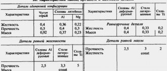
Modulus of elasticity of various materials

Elastic moduli for different materials have completely different values, which depend on:

• the nature of the substances that form the composition of the material;
• mono- or multicomponent composition (pure substance, alloy, etc.);
• structures (metallic or other type of crystal lattice, molecular structure, etc.);
• density of the material (distribution of particles in its volume);
• the processing to which it was subjected (firing, etching, pressing, etc.).

For example, in the reference data you can find that the elastic modulus for aluminum is in the range from 61.8 to 73.6 GPa. Apparently, this depends on the state of the metal and the type of processing, because for annealed aluminum the Young’s modulus is 68.5 GPa.

Its significance for bronze materials depends not only on the processing, but also on the chemical composition:

• bronze – 10.4 GPa;
• aluminum bronze during casting – 10.3 GPa;
• rolled phosphor bronze – 11.3 GPa.

Young's modulus of brass is much lower - 78.5-98.1. Rolled brass has the maximum value.

Copper itself in its pure form is characterized by a resistance to external influences that is much greater than its alloys - 128.7 GPa. Processing it also reduces the indicator, including rolling:

• cast – 82 GPa;
• rolled – 108 GPa;
• deformed – 112 GPa;
• cold drawn – 127 GPa.

Titanium (108 GPa), which is considered one of the strongest metals, has a value close to copper. But heavy but brittle lead shows only 15.7-16.2 GPa, which is comparable to the strength of wood.

For iron, the stress-to-strain ratio also depends on the method of its processing: cast - 100-130 or forged - 196.2-215.8 GPa.

Cast iron is known for its brittleness and has a stress-to-strain ratio of 73.6 to 150 GPa, which is consistent with its type. Whereas for steel, the elastic modulus can reach 235 GPa.

Elastic moduli of some materials

The values ​​of strength parameters are also influenced by the shape of the products. For example, for a steel rope, calculations are carried out, which take into account:

• its diameter;
• lay pitch;
• lay angle.

Interestingly, this figure for a rope will be significantly lower than for a wire of the same diameter.

It is worth noting the strength and non-metallic materials. For example, among the Young's moduli of wood, pine has the lowest - 8.8 GPa, but the group of hardwoods, which are united under the name "iron wood", has the highest - 32.5 GPa, oak and beech have equal indicators - 16.3 GPa.

Among building materials, the resistance to external forces of seemingly durable granite is only 35-50 GPa, while even glass is 78 GPa. Concrete is inferior to glass - up to 40 GPa, limestone and marble, with values ​​of 35 and 50 GPa, respectively.

Flexible materials such as rubber can withstand axial loads ranging from 0.0015 to 0.0079 GPa.

Links[edit]

1. "Volume elastic properties". hyperphysics
   . Georgia State University.
2. "Silicon rubber". AZO materials
   .
3. Page 52 of Introduction to Solid State Physics, 8th Edition by Charles Kittel, 2005, ISBN 0-471-41526-X
4. Flügel, Alexander. "Calculation of the volumetric modulus of glass". glassproperties.com
   .
5. H., Courtney, Thomas (2013). Mechanical behavior of materials
   (2nd ed. Reimp ed.). New Delhi: McGraw Hill Education (India). ISBN 978-1259027512. OCLC 929663641.
6. Jump up
   ↑ Gilman, J. J. (1969).
   Micromechanics of flow in solids
   . New York: McGraw-Hill. paragraph 29.

Further reading[edit]

• De Jong, Martin; Chen, Wei (2015). "Diagram of the total elastic properties of inorganic crystalline compounds". Scientific data
  .
  2
  : 150009. Bibcode: 2013NatSD...2E0009D. DOI: 10.1038/sdata.2015.9. PMC 4432655. PMID 25984348.