MAGNETS AND MAGNETIC PROPERTIES OF SUBSTANCE.
The simplest manifestations of magnetism have been known for a very long time and are familiar to most of us.
However, it was only relatively recently that these seemingly simple phenomena were explained based on the fundamental principles of physics. Also on topic:
MAGNETIC RESONANCE
There are two different types of magnets. Some are so-called permanent magnets, made from “hard magnetic” materials. Their magnetic properties are not related to the use of external sources or currents. Another type includes the so-called electromagnets with a core made of “soft magnetic” iron. The magnetic fields they create are mainly due to the fact that an electric current passes through the winding wire surrounding the core.
Magnetic poles and magnetic field.
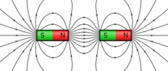
The magnetic properties of a bar magnet are most noticeable near its ends. If such a magnet is hung by the middle part so that it can rotate freely in a horizontal plane, then it will take a position approximately corresponding to the direction from north to south. The end of the rod pointing north is called the north pole, and the opposite end is called the south pole. Opposite poles of two magnets attract each other, and like poles repel each other.
Also on topic:
EARTH'S MAGNETIC FIELD
If a bar of non-magnetized iron is brought close to one of the poles of a magnet, the latter will become temporarily magnetized. In this case, the pole of the magnetized bar closest to the pole of the magnet will be opposite in name, and the far one will have the same name. The attraction between the pole of the magnet and the opposite pole induced by it in the bar explains the action of the magnet. Some materials (such as steel) themselves become weak permanent magnets after being near a permanent magnet or electromagnet. A steel rod can be magnetized by simply passing the end of a bar permanent magnet along its end.
So, a magnet attracts other magnets and objects made of magnetic materials without being in contact with them. This action at a distance is explained by the existence of a magnetic field in the space around the magnet. Some idea of the intensity and direction of this magnetic field can be obtained by pouring iron filings onto a sheet of cardboard or glass placed on a magnet. The sawdust will line up in chains in the direction of the field, and the density of the sawdust lines will correspond to the intensity of this field. (They are thickest at the ends of the magnet, where the intensity of the magnetic field is greatest.)
M. Faraday (1791–1867) introduced the concept of closed induction lines for magnets. The induction lines extend into the surrounding space from the magnet at its north pole, enter the magnet at its south pole, and pass inside the magnet material from the south pole back to the north, forming a closed loop. The total number of induction lines emerging from a magnet is called magnetic flux. Magnetic flux density, or magnetic induction ( V
), is equal to the number of induction lines passing along the normal through an elementary area of unit size.
Magnetic induction determines the force with which a magnetic field acts on a current-carrying conductor located in it. If the conductor carrying current I
, is located perpendicular to the induction lines, then according to Ampere’s law the force
F
acting on the conductor is perpendicular to both the field and the conductor and is proportional to the magnetic induction, current strength and length of the conductor.
Thus, for magnetic induction B
we can write the expression
where F
– force in newtons,
I
– current in amperes,
l
– length in meters. The unit of measurement for magnetic induction is tesla (T). See also ELECTRICITY AND MAGNETISM.
Characteristics of permanent magnet
- Magnetic force is characterized by residual magnetic induction. Designated Br. This is the force that remains after the disappearance of the external MP. Measured in tests (T) or gauss (G);
- Coercivity or resistance to demagnetization - Ns. Measured in A/m. Shows what the external MF intensity should be in order to demagnetize the material;
- Maximum energy – BHmax. Calculated by multiplying the remanent magnetic force Br and coercivity Hc. Measured in MGSE (megaussersted);
- Temperature coefficient of residual magnetic force – Тс of Br. Characterizes the dependence of Br on the temperature value;
- Tmax – the highest temperature value, upon reaching which permanent magnets lose their properties with the possibility of reverse recovery;
- Tcur is the highest temperature value at which the magnetic material irreversibly loses its properties. This indicator is called the Curie temperature.
Magnetic flux formula
Individual magnet characteristics change depending on temperature. At different temperatures, different types of magnetic materials perform differently.
Important! All permanent magnets lose a percentage of their magnetism as the temperature rises, but at different rates depending on their type.
Magnetizing force and magnetic field strength.
Next, we should introduce another quantity characterizing the magnetic effect of electric current. Suppose that current passes through the wire of a long coil, inside of which there is a magnetizable material. The magnetizing force is the product of the electric current in the coil and the number of its turns (this force is measured in amperes, since the number of turns is a dimensionless quantity). Magnetic field strength H
equal to the magnetizing force per unit length of the coil.
Thus, the value of H
is measured in amperes per meter; it determines the magnetization acquired by the material inside the coil.
In a vacuum, magnetic induction B
proportional to the magnetic field strength
H
:
where m
0 – so-called
magnetic constant having a universal value of 4 p
× 10–7 H/m.
In many materials, the value of
B
is
approximately proportional
to H. However, in ferromagnetic materials the relationship between B
and
H
is somewhat more complex (as will be discussed below).
In Fig. 1 shows a simple electromagnet designed to grip loads. The energy source is a DC battery. The figure also shows the field lines of the electromagnet, which can be detected by the usual method of iron filings.
Large electromagnets with iron cores and a very large number of ampere-turns, operating in continuous mode, have a large magnetizing force. They create a magnetic induction of up to 6 Tesla in the gap between the poles; this induction is limited only by mechanical stress, heating of the coils and magnetic saturation of the core. A number of giant water-cooled electromagnets (without a core), as well as installations for creating pulsed magnetic fields, were designed by P.L. Kapitsa (1894–1984) in Cambridge and at the Institute of Physical Problems of the USSR Academy of Sciences and F. Bitter (1902–1967) in Massachusetts Institute of Technology. With such magnets it was possible to achieve induction of up to 50 Tesla. A relatively small electromagnet that produces fields of up to 6.2 Tesla, consumes 15 kW of electrical power and is cooled by liquid hydrogen, was developed at the Losalamos National Laboratory. Similar fields are obtained at cryogenic temperatures.
Ferromagnets
There is a small group of substances that, due to their structural features, have very high magnetic properties. The first metal in which these qualities were discovered was iron, and thanks to it this group received the name ferromagnets.
The structure of ferromagnets is characterized by the presence of special structures - domains. These are areas where magnetization forms spontaneously. Due to the peculiarities of interatomic and intermolecular interactions in ferromagnets, the most energetically favorable arrangement of atomic and electronic magnetic moments is established. They acquire a parallel orientation along the so-called directions of easy magnetization. However, the entire volume of, for example, an iron crystal cannot acquire unidirectional spontaneous magnetization - this would increase the total energy of the system. Therefore, the system is divided into sections, the spontaneous magnetization of which in the ferromagnetic body compensates for each other. This is how domains are formed.
The magnetic susceptibility of ferromagnets is extremely high, can range from several tens to hundreds of thousands and largely depends on the strength of the external field. The reason for this is that the orientation of domains along the field direction also turns out to be energetically favorable. The direction of the magnetization vector of some domains will necessarily coincide with the field strength vector, and their energy will be the least. Such areas grow, and at the same time, unfavorably oriented domains shrink. Magnetization increases and magnetic induction increases. The process occurs unevenly, and the graph of the relationship between induction and external field strength is called the magnetization curve of a ferromagnetic substance.
When the temperature rises to a certain threshold value, called the Curie point, the domain structure is disrupted due to increased thermal motion. Under these conditions, the ferromagnet exhibits paramagnetic properties.
In addition to iron and steel, ferromagnetic properties are inherent in cobalt and nickel, some alloys and rare earth metals.
Tags: , automatic, ampere, sconce, gimlet, view, alignment, generator, hysteresis, engine, house, , sign, like, computer, , magnet, magnetic, permanent, potential, rule, principle, wire, start, , work, resonance, rheostat, row, system, resistance, circuit, ten, type, current, , installation, photo, hall, stepper, electric motor, electronic, effect
Magnetic permeability and its role in magnetism.
Magnetic permeability m
is a quantity characterizing the magnetic properties of a material.
Ferromagnetic metals Fe, Ni, Co and their alloys have very high maximum permeabilities - from 5000 (for Fe) to 800,000 (for supermalloy). In such materials, at relatively low field strengths H,
B
arise , but the relationship between these quantities, generally speaking, is nonlinear due to the phenomena of saturation and hysteresis, which are discussed below.
Ferromagnetic materials are strongly attracted by magnets. They lose their magnetic properties at temperatures above the Curie point (770° C for Fe, 358° C for Ni, 1120° C for Co) and behave like paramagnets, for which the induction B
up to very high strength values
H
is proportional to it - in exactly the same as what happens in a vacuum. Many elements and compounds are paramagnetic at all temperatures. Paramagnetic substances are characterized by the fact that they become magnetized in an external magnetic field; if this field is turned off, the paramagnetic substances return to a non-magnetized state. Magnetization in ferromagnets is maintained even after the external field is turned off.
In Fig. Figure 2 shows a typical hysteresis loop for a magnetically hard (with large losses) ferromagnetic material. It characterizes the ambiguous dependence of the magnetization of a magnetically ordered material on the strength of the magnetizing field. With increasing magnetic field strength from the initial (zero) point ( 1
) magnetization occurs along the dashed line
1
–
2
, and the value of
m
changes significantly as the magnetization of the sample increases.
At point 2
saturation is achieved, i.e.
with a further increase in voltage, the magnetization no longer increases. If we now gradually reduce the value of H
to zero, then the curve
B
(
H
) no longer follows the previous path, but passes through point
3
, revealing, as it were, a “memory” of the material about “past history,” hence the name “hysteresis.”
It is obvious that in this case some residual magnetization is retained (segment 1
–
3
).
After changing the direction of the magnetizing field to the opposite, the B
(
H
) curve passes point
4
, and the segment (
1
)–(
4
) corresponds to the coercive force that prevents demagnetization.
A further increase in the values (- H
) brings the hysteresis curve to the third quadrant - section
4
-
5
.
The subsequent decrease in the value (-H )
to zero and then an increase in positive values
of H
will lead to the closure of the hysteresis loop through points
6
,
7
and
2
.
Hard magnetic materials are characterized by a wide hysteresis loop, covering a significant area on the diagram and therefore corresponding to large values of remanent magnetization (magnetic induction) and coercive force. A narrow hysteresis loop (Fig. 3) is characteristic of soft magnetic materials, such as mild steel and special alloys with high magnetic permeability. Such alloys were created with the aim of reducing energy losses caused by hysteresis. Most of these special alloys, like ferrites, have high electrical resistance, which reduces not only magnetic losses, but also electrical losses caused by eddy currents.
Magnetic materials with high permeability are produced by annealing, carried out by holding at a temperature of about 1000 ° C, followed by tempering (gradual cooling) to room temperature. In this case, preliminary mechanical and thermal treatment, as well as the absence of impurities in the sample, are very important. For transformer cores at the beginning of the 20th century. silicon steels were developed, the value m
which increased with increasing silicon content.
Between 1915 and 1920, permalloys (alloys of Ni and Fe) appeared with a characteristic narrow and almost rectangular hysteresis loop. by especially high values of magnetic permeability m
at low values of
H
, while in perminvar (45 % Ni, 30% Fe, 25% Co) the value of
m
is practically constant over a wide range of changes in field strength. Among modern magnetic materials, mention should be made of supermalloy, an alloy with the highest magnetic permeability (it contains 79% Ni, 15% Fe and 5% Mo).
Diamagnetism
Diamagnetism occurs in all materials and is the tendency of a material to resist an applied magnetic field and therefore be repelled by a magnetic field. However, in a material with paramagnetic properties (that is, with a tendency to amplify an external magnetic field), paramagnetic behavior dominates. Thus, despite its universal occurrence, diamagnetic behavior is only observed in purely diamagnetic material. There are no unpaired electrons in a diamagnetic material, so the electrons' own magnetic moments cannot create any volume effect.
Please note that this description is intended as a heuristic only. The Bohr-van Leeuwen theorem shows that diamagnetism is impossible according to classical physics, and that a proper understanding requires a quantum mechanical description
Please note that all materials undergo this orbital response. However, in paramagnetic and ferromagnetic substances, the diamagnetic effect is suppressed by much stronger effects caused by unpaired electrons
A paramagnetic material has unpaired electrons; that is, atomic or molecular orbitals with exactly one electron in them. While the Pauli exclusion principle requires paired electrons to have their own ("spin") magnetic moments pointing in opposite directions, causing their magnetic fields to cancel out, an unpaired electron can align its magnetic moment in either direction. When an external field is applied, these moments will tend to align in the same direction as the applied field, enhancing it.
Theories of magnetism.
For the first time, the guess that magnetic phenomena are ultimately reduced to electrical phenomena arose from Ampere in 1825, when he expressed the idea of closed internal microcurrents circulating in each atom of a magnet. However, without any experimental confirmation of the presence of such currents in matter (the electron was discovered by J. Thomson only in 1897, and the description of the structure of the atom was given by Rutherford and Bohr in 1913), this theory “faded.” In 1852, W. Weber suggested that each atom of a magnetic substance is a tiny magnet, or magnetic dipole, so that complete magnetization of a substance is achieved when all individual atomic magnets are aligned in a certain order (Fig. 4, b
). Weber believed that molecular or atomic “friction” helps these elementary magnets maintain their order despite the disturbing influence of thermal vibrations. His theory was able to explain the magnetization of bodies upon contact with a magnet, as well as their demagnetization upon impact or heating; finally, the “reproduction” of magnets when cutting a magnetized needle or magnetic rod into pieces was also explained. And yet this theory did not explain either the origin of the elementary magnets themselves, or the phenomena of saturation and hysteresis. Weber's theory was improved in 1890 by J. Ewing, who replaced his hypothesis of atomic friction with the idea of interatomic confining forces that help maintain the ordering of the elementary dipoles that make up a permanent magnet.
The approach to the problem, once proposed by Ampere, received a second life in 1905, when P. Langevin explained the behavior of paramagnetic materials by attributing to each atom an internal uncompensated electron current. According to Langevin, it is these currents that form tiny magnets that are randomly oriented when there is no external field, but acquire an orderly orientation when it is applied. In this case, the approach to complete order corresponds to saturation of magnetization. In addition, Langevin introduced the concept of a magnetic moment, which for an individual atomic magnet is equal to the product of the “magnetic charge” of a pole and the distance between the poles. Thus, the weak magnetism of paramagnetic materials is due to the total magnetic moment created by uncompensated electron currents.
In 1907, P. Weiss introduced the concept of “domain,” which became an important contribution to the modern theory of magnetism. Weiss imagined domains as small “colonies” of atoms, within which the magnetic moments of all atoms, for some reason, are forced to maintain the same orientation, so that each domain is magnetized to saturation. An individual domain can have linear dimensions of the order of 0.01 mm and, accordingly, a volume of the order of 10–6 mm3. The domains are separated by so-called Bloch walls, the thickness of which does not exceed 1000 atomic sizes. The “wall” and two oppositely oriented domains are shown schematically in Fig. 5. Such walls represent “transition layers” in which the direction of domain magnetization changes.
In the general case, three sections can be distinguished on the initial magnetization curve (Fig. 6). In the initial section, the wall, under the influence of an external field, moves through the thickness of the substance until it encounters a defect in the crystal lattice, which stops it. By increasing the field strength, you can force the wall to move further, through the middle section between the dashed lines. If after this the field strength is again reduced to zero, then the walls will no longer return to their original position, so the sample will remain partially magnetized. This explains the hysteresis of the magnet. At the final section of the curve, the process ends with the saturation of the magnetization of the sample due to the ordering of the magnetization inside the last disordered domains. This process is almost completely reversible. Magnetic hardness is exhibited by those materials whose atomic lattice contains many defects that impede the movement of interdomain walls. This can be achieved by mechanical and thermal treatment, for example by compression and subsequent sintering of the powdered material. In alnico alloys and their analogues, the same result is achieved by fusing metals into a complex structure.
In addition to paramagnetic and ferromagnetic materials, there are materials with so-called antiferromagnetic and ferrimagnetic properties. The difference between these types of magnetism is explained in Fig. 7. Based on the concept of domains, paramagnetism can be considered as a phenomenon caused by the presence in the material of small groups of magnetic dipoles, in which individual dipoles interact very weakly with each other (or do not interact at all) and therefore, in the absence of an external field, take only random orientations ( Fig. 7, a
).
In ferromagnetic materials, within each domain there is a strong interaction between individual dipoles, leading to their ordered parallel alignment (Fig. 7, b
).
In antiferromagnetic materials, on the contrary, the interaction between individual dipoles leads to their antiparallel ordered alignment, so that the total magnetic moment of each domain is zero (Fig. 7c )
.
Finally, in ferrimagnetic materials (for example, ferrites) there is both parallel and antiparallel ordering (Fig. 7, d
), which results in weak magnetism.
There are two convincing experimental confirmations of the existence of domains. The first of them is the so-called Barkhausen effect, the second is the method of powder figures. In 1919, G. Barkhausen established that when an external field is applied to a sample of ferromagnetic material, its magnetization changes in small discrete portions. From the point of view of domain theory, this is nothing more than an abrupt advance of the interdomain wall, encountering on its way individual defects that delay it. This effect is usually detected using a coil in which a ferromagnetic rod or wire is placed. If you alternately bring a strong magnet towards and away from the sample, the sample will be magnetized and remagnetized. Abrupt changes in the magnetization of the sample change the magnetic flux through the coil, and an induction current is excited in it. The voltage generated in the coil is amplified and fed to the input of a pair of acoustic headphones. Clicks heard through headphones indicate an abrupt change in magnetization.
To reveal the domain structure of a magnet using the powder figure method, a drop of a colloidal suspension of ferromagnetic powder (usually Fe3O4) is applied to a well-polished surface of a magnetized material. Powder particles settle mainly in places of maximum inhomogeneity of the magnetic field - at the boundaries of domains. This structure can be studied under a microscope. A method based on the passage of polarized light through a transparent ferromagnetic material has also been proposed.
Weiss's original theory of magnetism in its main features has retained its significance to this day, having, however, received an updated interpretation based on the idea of uncompensated electron spins as a factor determining atomic magnetism. The hypothesis about the existence of an electron’s own momentum was put forward in 1926 by S. Goudsmit and J. Uhlenbeck, and at present it is electrons as spin carriers that are considered “elementary magnets”.
To explain this concept, consider (Fig. a free atom of iron, a typical ferromagnetic material. Its two shells ( K
and
L
), those closest to the nucleus, are filled with electrons, with the first of them containing two and the second containing eight electrons.
In the K
shell, the spin of one of the electrons is positive and the other is negative.
In the L
shell (more precisely, in its two subshells), four of the eight electrons have positive spins, and the other four have negative spins.
In both cases, the electron spins within one shell are completely compensated, so that the total magnetic moment is zero. In the M
shell the situation is different, since out of the six electrons located in the third subshell, five electrons have spins directed in one direction, and only the sixth in the other.
As a result, four uncompensated spins remain, which determines the magnetic properties of the iron atom. (There are only two valence electrons in the outer N
shell, which do not contribute to the magnetism of the iron atom.) The magnetism of other ferromagnets, such as nickel and cobalt, is explained in a similar way. Since neighboring atoms in an iron sample strongly interact with each other, and their electrons are partially collectivized, this explanation should be considered only as a visual, but very simplified diagram of the real situation.
The theory of atomic magnetism, based on taking into account the electron spin, is supported by two interesting gyromagnetic experiments, one of which was carried out by A. Einstein and W. de Haas, and the other by S. Barnett. In the first of these experiments, a cylinder of ferromagnetic material was suspended as shown in Fig. 9. If current is passed through the winding wire, the cylinder rotates around its axis. When the direction of the current (and therefore the magnetic field) changes, it turns in the opposite direction. In both cases, the rotation of the cylinder is due to the ordering of the electron spins. In Barnett's experiment, on the contrary, a suspended cylinder, sharply brought into a state of rotation, becomes magnetized in the absence of a magnetic field. This effect is explained by the fact that when the magnet rotates, a gyroscopic moment is created, which tends to rotate the spin moments in the direction of its own axis of rotation.
For a more complete explanation of the nature and origin of short-range forces that order neighboring atomic magnets and counteract the disordering influence of thermal motion, one should turn to quantum mechanics. A quantum mechanical explanation of the nature of these forces was proposed in 1928 by W. Heisenberg, who postulated the existence of exchange interactions between neighboring atoms. Later, G. Bethe and J. Slater showed that exchange forces increase significantly with decreasing distance between atoms, but upon reaching a certain minimum interatomic distance they drop to zero.
A little bit of history
People have been studying the properties of permanent magnets since very, very ancient times. They are mentioned in the works of scientists of Ancient Greece as far back as 600 years BC. Natural (naturally occurring) magnets can be found in magnetic ore deposits. The most famous of the large natural magnets is kept at the University of Tartu. It weighs 13 kilograms, and the load that can be lifted with its help is 40 kg.
Humanity has learned to create artificial magnets using various ferromagnets. The value of powdered ones (made of cobalt, iron, etc.) lies in the ability to hold a load weighing 5000 times its own weight. Artificial specimens can be permanent (obtained from hard magnetic materials) or electromagnets having a core made of soft magnetic iron. The voltage field in them arises due to the passage of electric current through the wires of the winding, which surrounds the core.
The first serious book containing attempts to scientifically study the properties of a magnet is the work of the London physician Gilbert, published in 1600. This work contains the entire set of information available at that time regarding magnetism and electricity, as well as the author’s experiments.
Man tries to adapt any of the existing phenomena to practical life. Of course, the magnet was no exception.
MAGNETIC PROPERTIES OF SUBSTANCE
One of the first extensive and systematic studies of the magnetic properties of matter was undertaken by P. Curie. He established that, according to their magnetic properties, all substances can be divided into three classes. The first category includes substances with pronounced magnetic properties, similar to the properties of iron. Such substances are called ferromagnetic; their magnetic field is noticeable at considerable distances ( cm
.
higher
). The second class includes substances called paramagnetic; Their magnetic properties are generally similar to those of ferromagnetic materials, but much weaker. For example, the force of attraction to the poles of a powerful electromagnet can tear an iron hammer out of your hands, and to detect the attraction of a paramagnetic substance to the same magnet, as a rule, you need very sensitive analytical balances. The last, third class includes the so-called diamagnetic substances. They are repelled by an electromagnet, i.e. the force acting on diamagnetic materials is directed opposite to that acting on ferro- and paramagnetic materials.
Measurement of magnetic properties.
When studying magnetic properties, two types of measurements are most important. The first of them is measuring the force acting on a sample near a magnet; This is how the magnetization of the sample is determined. The second includes measurements of “resonant” frequencies associated with the magnetization of matter. Atoms are tiny "gyros" and in a magnetic field precess (like a regular top under the influence of the torque created by gravity) at a frequency that can be measured. In addition, a force acts on free charged particles moving at right angles to the magnetic induction lines, just like the electron current in a conductor. It causes the particle to move in a circular orbit, the radius of which is given by
R
=
mv
/
eB
,
where m
is the mass of the particle,
v
is its speed,
e
is its charge, and
B
is the magnetic induction of the field. The frequency of such circular motion is
where f
is measured in hertz,
e
- in coulombs,
m
- in kilograms,
B
- in teslas. This frequency characterizes the movement of charged particles in a substance located in a magnetic field. Both types of motion (precession and motion along circular orbits) can be excited by alternating fields with resonant frequencies equal to the “natural” frequencies characteristic of a given material. In the first case, the resonance is called magnetic, and in the second - cyclotron (due to its similarity with the cyclic motion of a subatomic particle in a cyclotron).
Speaking about the magnetic properties of atoms, it is necessary to pay special attention to their angular momentum. The magnetic field acts on the rotating atomic dipole, tending to rotate it and place it parallel to the field. Instead, the atom begins to precess around the direction of the field (Fig. 10) with a frequency depending on the dipole moment and the strength of the applied field.
Atomic precession is not directly observable because all atoms in a sample precess at a different phase. If we apply a small alternating field directed perpendicular to the constant ordering field, then a certain phase relationship is established between the precessing atoms and their total magnetic moment begins to precess with a frequency equal to the precession frequency of individual magnetic moments. The angular velocity of precession is important. Typically, this value is on the order of 1010 Hz/T for magnetization associated with electrons, and on the order of 107 Hz/T for magnetization associated with positive charges in the nuclei of atoms.
A schematic diagram of a setup for observing nuclear magnetic resonance (NMR) is shown in Fig. 11. The substance being studied is introduced into a uniform constant field between the poles. If a radiofrequency field is then excited using a small coil surrounding the test tube, a resonance can be achieved at a specific frequency equal to the precession frequency of all nuclear “gyros” in the sample. The measurements are similar to tuning a radio receiver to the frequency of a specific station.
Magnetic resonance methods make it possible to study not only the magnetic properties of specific atoms and nuclei, but also the properties of their environment. The fact is that magnetic fields in solids and molecules are inhomogeneous, since they are distorted by atomic charges, and the details of the experimental resonance curve are determined by the local field in the region where the precessing nucleus is located. This makes it possible to study the structural features of a particular sample using resonance methods.
What else?
We humans are no exception. Thanks to the biocurrents flowing in the body, there is an invisible pattern of its power lines around us. Planet Earth is a huge magnet. And even more grandiose is the plasma ball of the sun. The dimensions of galaxies and nebulae, incomprehensible to the human mind, rarely allow the idea that all of these are also magnets.
Modern science requires the creation of new large and super-powerful magnets, the areas of application of which are related to thermonuclear fusion, generation of electrical energy, acceleration of charged particles in synchrotrons, and recovery of sunken ships. Creating a super-strong field using the magnetic properties of a magnet is one of the tasks of modern physics.